Homework Problems:
Quadrature
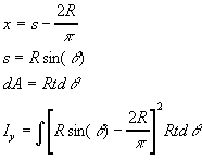
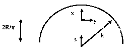
- The moment of inertia about the y-axis of the thin ring shown below can be represented
by :

Using a series of substitutions leads to an integral in the angle:

Here t is the thickness of the ring. Evaluate this last integral numerically for R=0.2 m and t=0.005 m. The handbook value for this integral is
 . I want you to solve this problem using both the trapezoidal and
Simpson's rules, and for each one you should use at least two different mesh sizes.
- Find the average value of the simple Gaussian distribution represented by the function
below on the interval -1 < x < 1.

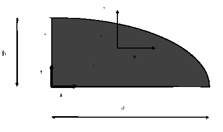
- Find the moment of inertia about the y-axis of the quarter-ellipse shown below, using a=20
cm and b=10 cm. This quantity can be defined by the following intergral:


- Use Monte Carlo integration to find the area of the quarter-ellipse in problem 3.
- Use Monte Carlo integration to find the moment of inertia that you calculated in problem
3. Note that the moment of inertia is defined as:

- Integration: Trapezoidal and Simpson's Rule
Most numerical schemes for integration divide an interval into pieces [as determined by the abscissa values ] and approximate the function as
a weighted sum of function evaluations at those abscissa points. This can be summarized
as:
where the
 are constants, called weights. The two
most common approaches are the trapezoidal rule and Simpson's rule. Each of these divide
the interval up into N even pieces and choose different sets of weights. The
trapezoidal rule gives:
where

and

Simpson's rule gives:


- Use both these techniques to do the integral below and compare the accuracies.

- Now repeat the previous question using twice as many mesh points and compare the accuracies.
- Use both these techniques to do the integral below and compare the accuracies.
- Integration: the error function
Using the trapezoidal rule, determine the number of mesh points that are required to do the integral below with an accuracy of at least .
. 
This integral is related to the error function [referred to as erf(z)], because

- Consider the function:

Plot this function on the interval 0<x<1. (beware of singularities!) By looking at this plot, make an estimate for:

Now determine this integral numerically (using whatever method you prefer) and compare the result to your estimate.
- Integration: Monte Carlo
Use Monte Carlo integration to determine the integral
- What is the relative error when you use 500 points?
- What is the relative error when you use 1,000 points?
- Integration: Gaussian Quadrature
Gaussian Quadrature is a numerical integration technique. In this case, we represent the integral by:
where

with the weights and abscissa values defined accordingly. A significant difference between this technique and others is that the abscissa values
 are not evenly spaced. For 8-point Gauss Quadrature, the weights and
abscissas are:

-0.960289856497536 0.101228536290376 -0.796666477413627 0.222381034453374 -0.525532409916329 0.313706645877887 -0.183434642495650 0.362683783378362 0.183434642495650 0.362683783378362 0.525532409916329 0.313706645877887 0.796666477413627 0.222381034453374 0.960289856497536 0.101228536290376 Use 8-point Gauss quadrature to calculate the integral from problem 8 and compare your results.