In this section, we will discuss three topics associated with solving elliptic partial differential equations:
- Finite Difference Techniques
- Successive Overrelaxation
- Plate Theory
2-D Boundary Value Problems:
Finite Difference Techniques
Here we switch from studying 1-D boundary value problems to 2-D problems. Thus there are two independent variables (typically x and y or r and ) and our ordinary differential equations become partial differential equations (PDE's). There are many types of partial differential equations; we will begin with elliptic equations. For our purposes, we will consider elliptic equations to be equations for which the independent variables are both spatial (as opposed to temporal), so that we consider closed, 2-D regions in space with boundary appropriately provided on all boundaries. Engineering examples of elliptic PDE's include heat conduction, diffusion, electric fields, and torsion. We will deal, initially, with heat conduction problems in two dimensions. In these problems, we will seek solutions for the temperature field in some 2-D region with specified boundary conditions. The governing equation for these problems is:
![]()
where T is the temperature, Q is the volumetric heating, and k is the thermal conductivity of the solid. In Cartesian coordinates this equation becomes:
![]()
while in polar coordinates the governing equation is:
![]()
or
![]() .
.
As a model problem, we'll consider a rectangular plate of width a and height b, so our region of interest is the rectangle defined by: 0<x<a and 0<y<b. For boundary conditions, we will assume we know the temperature along the entire boundary of this plate. These are known as Dirichlet boundary conditions. We will assume that the temperature on all the boundaries is zero, except for the boundary at y=0, on which we will assume the temperature to be T(x,0)=f(x), where f(x) is a known function. This equation can be solved using separation of variables, giving the solution:

To find the solution, we determine the coefficients ![]() and then sum the series for the temperature field. This is actually done more easily with
numerical methods.
and then sum the series for the temperature field. This is actually done more easily with
numerical methods.
To solve this problem numerically, we divide the rectangle into a grid and assign a
temperature to each grid point. This is the 2-D equivalent of dividing a 1-D region into
intervals to create mesh points. We will label each temperature using the notation ![]() , where i denotes the row number and j
denotes the column number. We will assume that the grid spacing in the x-direction
is given by h and the spacing in the y-direction is s. Given this
model, we can approximate the second partial derivative of the temperature with respect to
x as:
, where i denotes the row number and j
denotes the column number. We will assume that the grid spacing in the x-direction
is given by h and the spacing in the y-direction is s. Given this
model, we can approximate the second partial derivative of the temperature with respect to
x as:
![]()
and the second partial derivative of the temperature with respect to y as:
![]()
If we substitute these into our PDE and set Q=0, then we obtain:
![]()
Solving this for ![]() we obtain:
we obtain:
 .
.
For the case of equal mesh spacing in each direction, i.e. h=s, we obtain:
![]() .
.
In other words, the temperature at any mesh point is the average of its four nearest neighbors.
2-D Boundary Value Problems:
Speeding up the Convergence with Successive
Overrelaxation
Here we consider a way to accelerate the convergence of elliptic PDE's. The technique is called successive overrelaxation (SOR). I'll first look at a similar effect in one dimension to demonstrate the technique, and then I'll look at how you implement it for elliptic PDE's in Excel.
A 1-D Analog
Consider Newton's method for finding the roots of functions of one variable. As shown graphically below, this technique starts with a guess, extrapolates a tangent to the curve until it crosses the axis, and then uses this crossing point as a new guess. Note how the iteration underestimates the amount needed to reach the real root.

If we simply increase the correction by a predetermined factor, we can accelerate the convergence. Obviously, for some functions convergence would be harmed by increasing the increment prescribed by Newton's method, but for a large class of elliptic PDE's, the two-dimensional analog of this technique dramatically improves convergence.
Successive Overrelaxation
To demonstrate overrelaxation for elliptic PDE's, we'll consider the example discussed in the previous exercise. That is, we'll deal with heat conduction problems in two dimensions. The governing equation for these problems is:
![]()
where T is the temperature, Q is the volumetric heating, and k is the thermal conductivity of the solid. Differencing this equation and using equal mesh spacing in both directions yields:
![]() .
.
Now we must massage this equation to make it suitable for SOR. We do this by adding and subtracting a term from the right side of the equation, yielding
![]()
Written in this fashion, the second term on the right side of this equation can be thought of as the correction to the current guess. Next we add an overrelaxation parameter (), yielding:

For greater than 1, this provides overrelaxation.
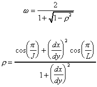
In order to yield optimum convergence, we must choose the value for the overrelaxation parameter that minimizes the number of iterations to convergence. For the classes of equations we've been considering, the optimal value is found from

where dx and dy are are the mesh spacings in the x and y
directions, respectively, J is the number of mesh points in the x direction,
and L is the number of points in the y direction.
Here we consider a a particular type of elliptic PDE: plate theory. The deformation of plates is governed by the following fourth-order PDE:
![]()
where w is the displacement of the plate, q is the transverse pressure applied to the plate, and
![]()
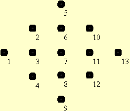
Here, E is the elastic modulus for the plate material, v is its Poisson's ratio, and h is the plate thickness. To difference this equation, it's convenient to number the mesh points in the neighborhood of a particular point. I'll use the following numbering scheme:

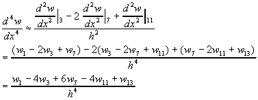
Our goal is a finite difference approximation to our PDE, written about point 7. We can write the first term as:

Similarly,

Substituting these into our PDE yields the following difference equation for the operator:

This can then be used to solve plate problems.