Curve-Fitting in Excel
We’ve seen the theory of curve-fitting by least squares methods, but we still must confront the details of implementation in Excel. We will look at two methods: use of the LINEST command and use of the Solver to do nonlinear fits.
Using LINEST
For doing linear fits, the LINEST command is a convenient way to obtain both the fitting parameters and appropriate statistics relevant to the fit. The syntax of the command is:
=LINEST(y-data, x-data, const, stats)
where y-data is a vector holding the data for the dependent variables, x-data is an array holding the data for the independent variable, as well as data for additional functions of the independent variable, and const and stats are boolean variables which are either TRUE of FALSE.
An important feature of the LINEST command is that it returns several values. Hence it must be handled somewhat differently from most other Excel functions. The process for using this command for curve-fitting can be summarized as:
- Put the data into the spreadsheet
- Highlight a block of cells, with the block consisting of 5 rows and one column for each parameter to be determined by the curve-fit
- Type in the LINEST function.
- Hit Control-Shift-Enter to obtain the results.
The actual use of this procedure will be demonstrated by a series of fits to the following data, which represents people’s heights as a function of their shoe sizes (men’s):
Shoe Size |
Height (inches) |
5.5 |
68.0 |
7.5 |
69.0 |
9.0 |
69.5 |
10.5 |
71.25 |
We will fit this to a straight line, a parabola, and a trigonometric function.
A straight-line fit
Here we fit the data to a straight line, so we have, as a model, H=aS+b, where H is the height and S is the shoe size. A spreadsheet for performing the curve fit is shown just below:

The LINEST formula that created the values in the above spreadsheet is:
=LINEST(B2:B5,A2:A5,TRUE,TRUE).
This formula was entered after highlighting cells E2:F6. The resulting model for height as a function of shoe size is H=64.44749+0.614155 S. Values for this model are generated in column C. The most important statistics are
- the errors in a and b (0.118 and 0.987), respectively. We want these to be small compared to a and b. In this case, the error in a is larger than we’d like, indicating a poor fit. To improve on this, we would have to choose a different model.
- The error expected for H (0.438). We want this to be small relative to the data for H, which it is.
- The value of r2 (0.9307), which should be as close to 1 as possible.
A parabolic fit
Here we fit the data to H=aS2+bS+c. Now we have 3 parameters, so we have 3 columns of results from LINEST. Also, we have to add a column for the square of the shoe size (S). When using LINEST, you need a column in the sheet for each term in the model that depends on the independent variable. In this case, we need columns for the first two terms in the model, because each depends on shoe size. The resulting spreadsheet is:

The LINEST formula that created the values in the above spreadsheet is:
=LINEST(A2:A5,B2:C5,TRUE,TRUE).
Note that here I’ve moved the height data into column A because all the shoe size data (S and S2) must be next to each other. Also, the shoe size data includes two columns, referred to here as B2:C5. The trick here is to connect the results of LINEST with the parameters in the model. The rule-of-thumb is: the constant is always in the right-most column (here 69.75274) and the next column (moving left) holds the constant for the data in the first column of x-data. That is, the value -0.79368 corresponds to the x-data in column B and thus represents b, the linear term. The remaining term, 0.08833, goes with column C and thus represents our constant a.
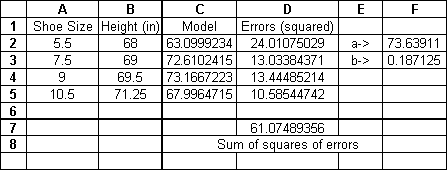
Curve-Fits "from scratch"
For doing nonlinear fits, we have to build our own curve-fit from scratch. As an example, suppose we want to fit our data to the function H=a sin(bS). To do this, follow the steps below:
- Put the data for H in column B and the data for S in column A.
- Put a guess for a in cell F2 and a guess for b in cell F3.
- In column C, generate model values for H using the guesses for a and b.
- In column D, generate the square of the error between the data for H and the value for H from the model (in column C)
- Sum up the squares of the errors
- Now use the Solver to minimize this sum by varying a and b.
My result of this process is given below:

Note here that the model I’ve chosen is not a particularly good one, and that other parameters (a and b) will likely give even lower residuals (errors). This is just meant to be a representative case.